TensorFlow实现非线性支持向量机的实现方法
这里将加载iris数据集,创建一个山鸢尾花(I.setosa)的分类器。
# Nonlinear SVM Example
#----------------------------------
#
# This function wll illustrate how to
# implement the gaussian kernel on
# the iris dataset.
#
# Gaussian Kernel:
# K(x1, x2) = exp(-gamma * abs(x1 - x2)^2)

import matplotlib.pyplot as plt
import numpy as np
import tensorflow as tf
from sklearn import datasets
from tensorflow.python.framework import ops
ops.reset_default_graph()

# Create graph
sess = tf.Session()

# Load the data
# iris.data = [(Sepal Length, Sepal Width, Petal Length, Petal Width)]
# 加载iris数据集,抽取花萼长度和花瓣宽度,分割每类的x_vals值和y_vals值
iris = datasets.load_iris()
x_vals = np.array([[x[0], x[3]] for x in iris.data])
y_vals = np.array([1 if y==0 else -1 for y in iris.target])
class1_x = [x[0] for i,x in enumerate(x_vals) if y_vals[i]==1]
class1_y = [x[1] for i,x in enumerate(x_vals) if y_vals[i]==1]
class2_x = [x[0] for i,x in enumerate(x_vals) if y_vals[i]==-1]
class2_y = [x[1] for i,x in enumerate(x_vals) if y_vals[i]==-1]

# Declare batch size
# 声明批量大小(偏向于更大批量大小)
batch_size = 150

# Initialize placeholders
x_data = tf.placeholder(shape=[None, 2], dtype=tf.float32)
y_target = tf.placeholder(shape=[None, 1], dtype=tf.float32)
prediction_grid = tf.placeholder(shape=[None, 2], dtype=tf.float32)

# Create variables for svm
b = tf.Variable(tf.random_normal(shape=[1,batch_size]))

# Gaussian (RBF) kernel
# 声明批量大小(偏向于更大批量大小)
gamma = tf.constant(-25.0)
sq_dists = tf.multiply(2., tf.matmul(x_data, tf.transpose(x_data)))
my_kernel = tf.exp(tf.multiply(gamma, tf.abs(sq_dists)))

# Compute SVM Model
first_term = tf.reduce_sum(b)
b_vec_cross = tf.matmul(tf.transpose(b), b)
y_target_cross = tf.matmul(y_target, tf.transpose(y_target))
second_term = tf.reduce_sum(tf.multiply(my_kernel, tf.multiply(b_vec_cross, y_target_cross)))
loss = tf.negative(tf.subtract(first_term, second_term))

# Gaussian (RBF) prediction kernel
# 创建一个预测核函数
rA = tf.reshape(tf.reduce_sum(tf.square(x_data), 1),[-1,1])
rB = tf.reshape(tf.reduce_sum(tf.square(prediction_grid), 1),[-1,1])
pred_sq_dist = tf.add(tf.subtract(rA, tf.multiply(2., tf.matmul(x_data, tf.transpose(prediction_grid)))), tf.transpose(rB))
pred_kernel = tf.exp(tf.multiply(gamma, tf.abs(pred_sq_dist)))

# 声明一个准确度函数,其为正确分类的数据点的百分比
prediction_output = tf.matmul(tf.multiply(tf.transpose(y_target),b), pred_kernel)
prediction = tf.sign(prediction_output-tf.reduce_mean(prediction_output))
accuracy = tf.reduce_mean(tf.cast(tf.equal(tf.squeeze(prediction), tf.squeeze(y_target)), tf.float32))

# Declare optimizer
my_opt = tf.train.GradientDescentOptimizer(0.01)
train_step = my_opt.minimize(loss)

# Initialize variables
init = tf.global_variables_initializer()
sess.run(init)

# Training loop
loss_vec = []
batch_accuracy = []
for i in range(300):
  rand_index = np.random.choice(len(x_vals), size=batch_size)
  rand_x = x_vals[rand_index]
  rand_y = np.transpose([y_vals[rand_index]])
  sess.run(train_step, feed_dict={x_data: rand_x, y_target: rand_y})

  temp_loss = sess.run(loss, feed_dict={x_data: rand_x, y_target: rand_y})
  loss_vec.append(temp_loss)

  acc_temp = sess.run(accuracy, feed_dict={x_data: rand_x,
                       y_target: rand_y,
                       prediction_grid:rand_x})
  batch_accuracy.append(acc_temp)

  if (i+1)%75==0:
    print('Step #' + str(i+1))
    print('Loss = ' + str(temp_loss))

# Create a mesh to plot points in
# 为了绘制决策边界(Decision Boundary),我们创建一个数据点(x,y)的网格,评估预测函数
x_min, x_max = x_vals[:, 0].min() - 1, x_vals[:, 0].max() + 1
y_min, y_max = x_vals[:, 1].min() - 1, x_vals[:, 1].max() + 1
xx, yy = np.meshgrid(np.arange(x_min, x_max, 0.02),
           np.arange(y_min, y_max, 0.02))
grid_points = np.c_[xx.ravel(), yy.ravel()]
[grid_predictions] = sess.run(prediction, feed_dict={x_data: rand_x,
                          y_target: rand_y,
                          prediction_grid: grid_points})
grid_predictions = grid_predictions.reshape(xx.shape)

# Plot points and grid
plt.contourf(xx, yy, grid_predictions, cmap=plt.cm.Paired, alpha=0.8)
plt.plot(class1_x, class1_y, 'ro', label='I. setosa')
plt.plot(class2_x, class2_y, 'kx', label='Non setosa')
plt.title('Gaussian SVM Results on Iris Data')
plt.xlabel('Pedal Length')
plt.ylabel('Sepal Width')
plt.legend(loc='lower right')
plt.ylim([-0.5, 3.0])
plt.xlim([3.5, 8.5])
plt.show()

# Plot batch accuracy
plt.plot(batch_accuracy, 'k-', label='Accuracy')
plt.title('Batch Accuracy')
plt.xlabel('Generation')
plt.ylabel('Accuracy')
plt.legend(loc='lower right')
plt.show()

# Plot loss over time
plt.plot(loss_vec, 'k-')
plt.title('Loss per Generation')
plt.xlabel('Generation')
plt.ylabel('Loss')
plt.show()
输出:
Step #75
Loss = -110.332
Step #150
Loss = -222.832
Step #225
Loss = -335.332
Step #300
Loss = -447.832
四种不同的gamma值(1,10,25,100):
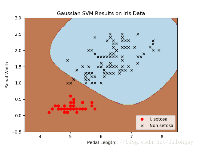
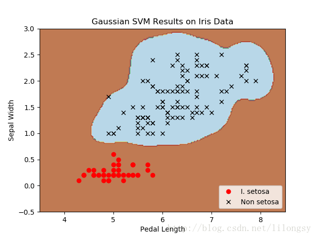
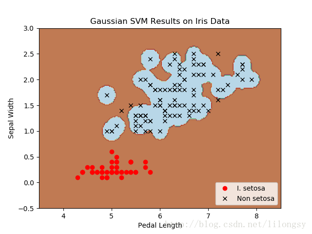
不同gamma值的山鸢尾花(I.setosa)的分类器结果图,采用高斯核函数的SVM。
gamma值越大,每个数据点对分类边界的影响就越大。
以上就是本文的全部内容,希望对大家的学习有所帮助,也希望大家多多支持【听图阁-专注于Python设计】。